Now we create a camera positioned so that it points directly down the z-axis at the origin.
We then create a plane positioned like a wall at z=0. This plane will completely fill the screen. It will be colored with white and gray wrinkles.
Finally, create a light source.
We render this scene at 640x480 +A0.1 +FT. We will get an image that will produce an excellent height field. We create a new file called hfdemo.pov and edit it as follows:
We add a camera that is two units above the origin and ten units back ...
... and a light source.
Now we add the height field. In the following syntax, a Targa image file is specified, the height field is smoothed, it is given a simple white pigment, it is translated to center it around the origin and it is scaled so that it resembles mountains and fills the screen.
We save the file and render it at 320x240 -A. Later, when we are satisfied that the height field is the way we want it, we render it at a higher resolution with anti-aliasing.
Wow! The Himalayas have come to our computer screen!
Here is some source for a really basic lathe (called lathdem1.pov).
We render this, and what we see is a fairly simply type of lathe, which looks like a child's top. Let's take a look at how this code produced the effect.
First, a set of six points are declared which the raytracer connects with lines. We note that there are only two components in the vectors which describe these points. The lines that are drawn are assumed to be in the x-y-plane, therefore it is as if all the z-components were assumed to be zero. The use of a two-dimensional vector is mandatory (Attempting to use a 3D vector would trigger an error... with one exception, which we will explore later in the discussion of splines).
Once the lines are determined, the ray-tracer rotates this line around the y-axis, and we can imagine a trail being left through space as it goes, with the surface of that trail being the surface of our object.
The specified points are connected with straight lines because we used the linear_spline keyword. There are other types of splines available with the lathe, which will result in smooth curving lines, and even rounded curving points of transition, but we will get back to that in a moment.
First, we would like to digress a moment to talk about the difference between a lathe and a surface of revolution object (SOR). The SOR object, described in a separate tutorial, may seem terribly similar to the lathe at first glance. It too declares a series of points and connects them with curving lines and then rotates them around the y-axis. The lathe has certain advantages, such as different kinds of splines, linear, quadratic and cubic, and one more thing:
The simpler mathematics used by a SOR doesn't allow the curve to double back over the same y-coordinates, thus, if using a SOR, any sudden twist which cuts back down over the same heights that the curve previously covered will trigger an error. For example, suppose we wanted a lathe to arc up from <0,0> to <2,2>, then to dip back down to <4,0>. Rotated around the y-axis, this would produce something like a gelatin mold - a rounded semi torus, hollow in the middle. But with the SOR, as soon as the curve doubled back on itself in the y-direction, it would become an illegal declaration.
Still, the SOR has one powerful strong point: because it uses simpler order mathematics, it generally tends to render faster than an equivalent lathe. So in the end, its a matter of: we use a SOR if its limitations will allow, but when we need a more flexible shape, we go with the lathe instead.
Now, we take a deep breath. We know that all looks a bit weird, but with some simple explanations, we can easily see what all this does.
First, we are using the orthographic camera. If we haven't read up on that yet, a quick summary is: it renders the scene flat, eliminating perspective distortion so that in a side view, the objects look like they were drawn on a piece of graph paper (like in the side view of a modeller or CAD package). There are several uses for this practical new type of camera, but here it is allowing us to see our lathe and cylinders edge on, so that what we see is almost like a cross section of the curve which makes the lathe, rather than the lathe itself. To further that effect, we eliminated shadowing with the ambient 1 finish, which of course also eliminates the need for lighting. We have also positioned this particular side view so that <0,0> appears at the lower left of our scene.
Next, we declared a set of points. We note that we used 3D vectors for these points rather than the 2D vectors we expect in a lathe. That's the exception we mentioned earlier. When we declare a 3D point, then use it in a lathe, the lathe only uses the first two components of the vector, and whatever is in the third component is simply ignored. This is handy here, since it makes this example possible.
Next we do two things with the declared points. First we use them to place small diameter cylinders at the locations of the points with the circular caps facing the camera. Then we re-use those same vectors to determine the lathe. Since trying to declare a 2D vector can have some odd results, and isn't really what our cylinder declarations need anyway, we can take advantage of the lathe's tendancy to ignore the third component by just setting the z-coordinate in these 3D vectors to zero.
The end result is: when we render this code, we see a white lathe against a black background showing us how the curve we've declared looks, and the circular ends of the cylinders show us where along the x-y-plane our control points are. In this case, it's very simple. The linear spline has been used so our curve is just straight lines zig-zagging between the points. We change the declarations of Red_Point and Blue_Point to read as follows (see file lathdem3.pov).
We re-render and, as we can see, all that happens is that the straight line segments just move to accomodate the new position of the red and blue points. Linear splines are so simple, we could manipulate them in our sleep, no?
Let's try something different. First, we change the points to the following (see file lathdem4.pov).
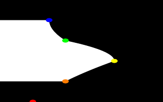
We then go down to the lathe declaration and change linear_spline to quadratic_spline. We re-render and what do we have? Well, there's a couple of things worthy of note this time. First, we will see that instead of straight lines we have smooth arcs connecting the points. These arcs are made from quadratic curves, so our lathe looks much more interesting this time. Also, Red_Point is no longer connected to the curve. What happened?
Well, while any two points can determine a straight line, it takes three to determine a quadratic curve. POV-Ray looks not only to the two points to be connected, but to the point immediately preceeding them to determine the formula of the quadratic curve that will be used to connect them. The problem comes in at the beginning of the curve. Beyond the first point in the curve there is no previous point. So we need to declare one. Therefore, when using a quadratic spline, we must remember that the first point we specify is only there so that POV-Ray can determine what curve to connect the first two points with. It will not show up as part of the actual curve.
There's just one more thing about this lathe example. Even though our curve is now put together with smooth curving lines, the transitions between those lines is... well, kind of choppy, no? This curve looks like the lines between each individual point have been terribly mismatched. Depending on what we are trying to make, this could be acceptable, or, we might long for a more smoothly curving shape. Fortunately, if the latter is true, we have another option.
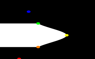
The quadratic spline takes longer to render than a linear spline. The math is more complex. Still longer needs the cubic spline, yet, for a really smoothed out shape, this is the only way to go. We go back into our example, and simply replace quadratic_spline with cubic_spline (see file lathdem5.pov). We render one more time, and take a look at what we have.
While a quadratic spline takes three points to determine the curve, a cubic needs four. So, as we might expect, Blue_Point has now dropped out of the curve, just as Red_Point did, as the first and last points of our curve are now only control points for shaping the curves between the remaining points. But look at the transition from Orange_Point to Yellow_Point and then back to Green_Point. Now, rather than looking mismatched, our curve segements look like one smoothly joined curve.
The concept of splines is a handy and necessary one, which will be seen again in the prism and polygon objects. But with a little tinkering we can quickly get a feel for working with them.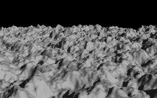
A height field created completely with POV-Ray.
Section 4.4.4
Lathe Object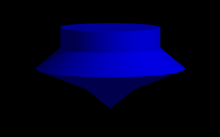
A simple lathe object.
Section 4.4.4.1
Understanding The Concept of Splines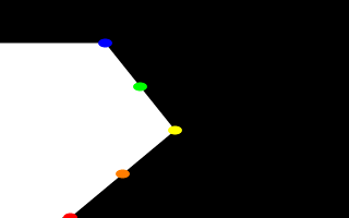
A simple "Spline Workshop".
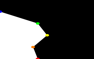
Moving some points of the spline.
A quadratic spline lathe.
A cubic spline lathe.
Table Of Contents